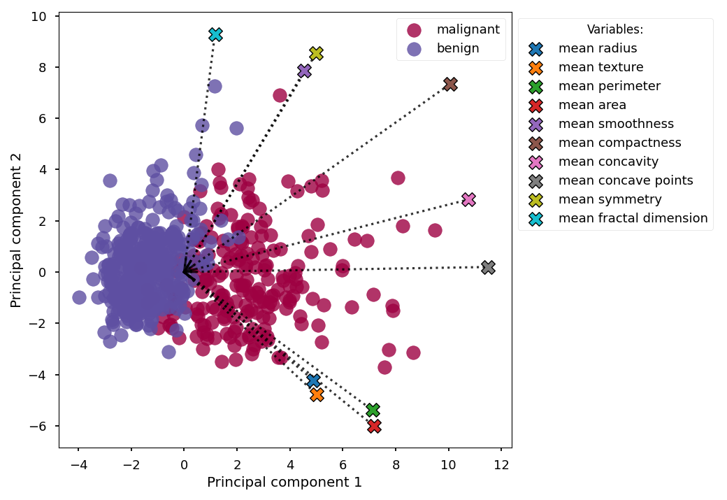
PCA Scores (2D) with loadings and a legend

This example will plot PCA scores along two principal axes and also show the loadings. Here we show labels in a legend, rather than in the plot, to avoid making the plot too crowded.

For better results, the parameter savefig can be used when calling pca_2d_scores() to store the plot directly to a (svg) file. In many cases, it is better to adjust the plot in an external tool, e.g. inkscape, to accompany all elements.

from matplotlib import pyplot as plt
import pandas as pd
from sklearn.datasets import load_breast_cancer
from sklearn.preprocessing import scale
from sklearn.decomposition import PCA
from psynlig import pca_2d_scores
plt.style.use('seaborn-talk')

data_set = load_breast_cancer()
data = pd.DataFrame(data_set['data'], columns=data_set['feature_names'])
xvars = [
    'mean radius',
    'mean texture',
    'mean perimeter',
    'mean area',
    'mean smoothness',
    'mean compactness',
    'mean concavity',
    'mean concave points',
    'mean symmetry',
    'mean fractal dimension',
]
data = data[xvars]
class_data = data_set['target']
class_names = dict(enumerate(data_set['target_names']))
data = scale(data)

pca = PCA()
scores = pca.fit_transform(data)

loading_settings = {
    'add_text': False,
    'add_legend': True,
}

pca_2d_scores(
    pca,
    scores,
    xvars=xvars,
    class_data=class_data,
    class_names=class_names,
    select_components={(1, 2)},
    loading_settings=loading_settings,
    s=200,
    alpha=.8,
    cmap_class='Spectral',
)

plt.show()