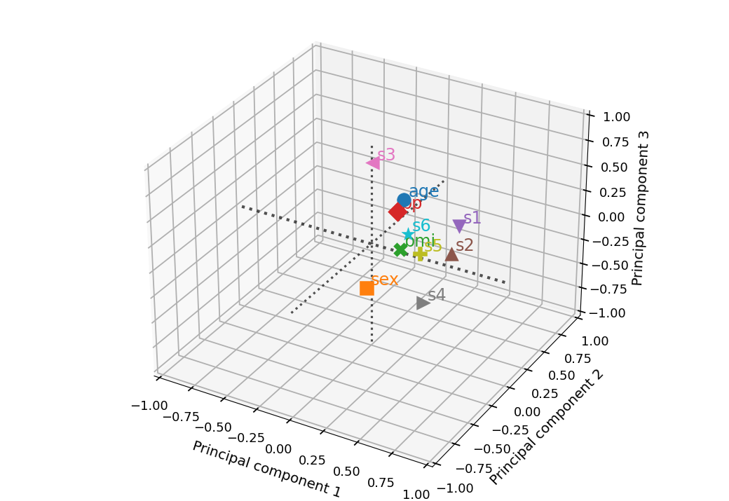
PCA Loadings (3D)

This example will plot PCA loadings along three principal axes.

• 
• 
• 

from matplotlib import pyplot as plt
import pandas as pd
from sklearn.datasets import load_diabetes
from sklearn.preprocessing import scale
from sklearn.decomposition import PCA
from psynlig import pca_3d_loadings
plt.style.use('seaborn-talk')

data_set = load_diabetes()
data = pd.DataFrame(data_set['data'], columns=data_set['feature_names'])
data = scale(data)

pca = PCA()
pca.fit_transform(data)


# Plot the loadings for 3 principal components:
pca_3d_loadings(
    pca,
    data_set['feature_names'],
    select_components={(1, 2, 3)}
)


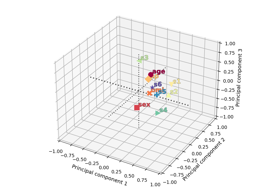
# Modify the text settings and plot the loadings
# for 3 principal components:
text_settings = {
    'fontsize': 'xx-large',
    'weight': 'bold',
    'outline': {'linewidth': 0.5}
}

pca_3d_loadings(
    pca,
    data_set['feature_names'],
    select_components={(1, 2, 3)},
    cmap='Spectral',
    text_settings=text_settings
)

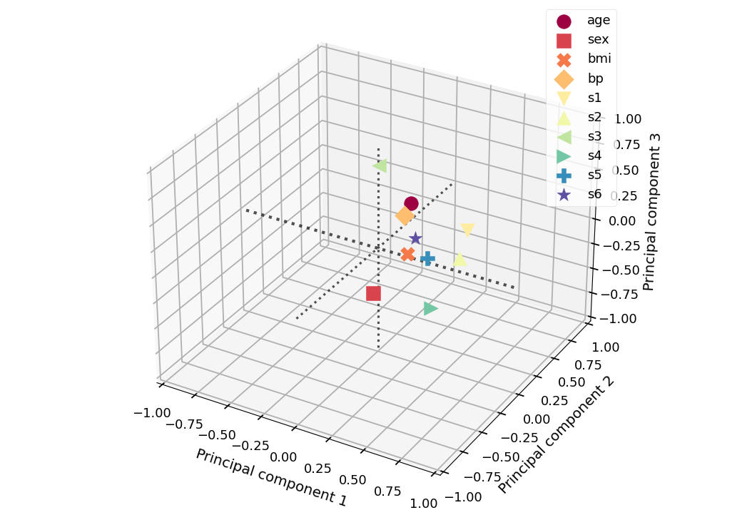
# Remove text from plot and add legend:
_, axes = pca_3d_loadings(
    pca,
    data_set['feature_names'],
    select_components={(1, 2, 3)},
    cmap='Spectral',
    text_settings={'show': False},
)
for axi in axes:
    axi.legend()

plt.show()